library(tidyverse)Normal quantile plots
The normal quantile plot
- see that normal distributions of data (or being normal enough) important
- only tools we have to assess this are histograms and maybe boxplots
- a better tool is normal quantile plot:
- plot data against what you expect if data actually normal
- look for points to follow a straight line, at least approx
ggplotcode:aessample; geomsstat_qqandstat_qq_line
Packages
The usual:
Kids learning to read
Rows: 44
Columns: 2
$ group <chr> "t", "t", "t", "t", "t", "t", "t", "t", "t", "t", "t", "t", "t",…
$ score <dbl> 24, 61, 59, 46, 43, 44, 52, 43, 58, 67, 62, 57, 71, 49, 54, 43, …ggplot(kids, aes(x = group, y = score)) + geom_boxplot()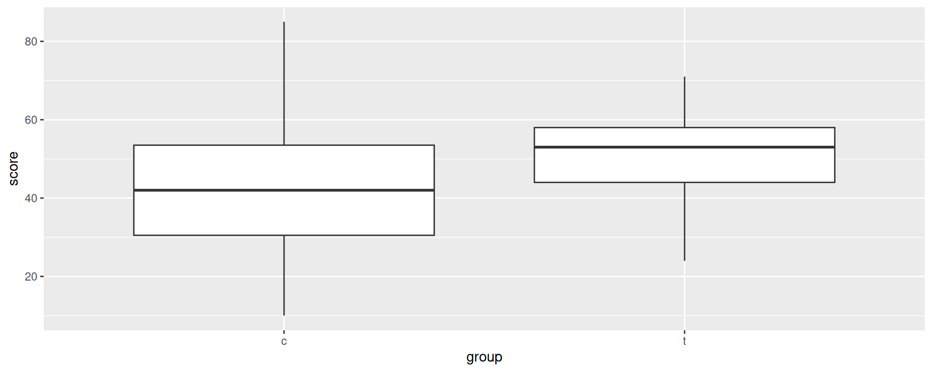
Groups look normal, at least close to symmetric.
Get the groups separately
kids %>% filter(group == "t") -> treatment
kids %>% filter(group == "c") -> control
to check
treatment %>% count(group)control %>% count(group)The treatment group
ggplot(treatment, aes(sample = score)) +
  stat_qq() + stat_qq_line()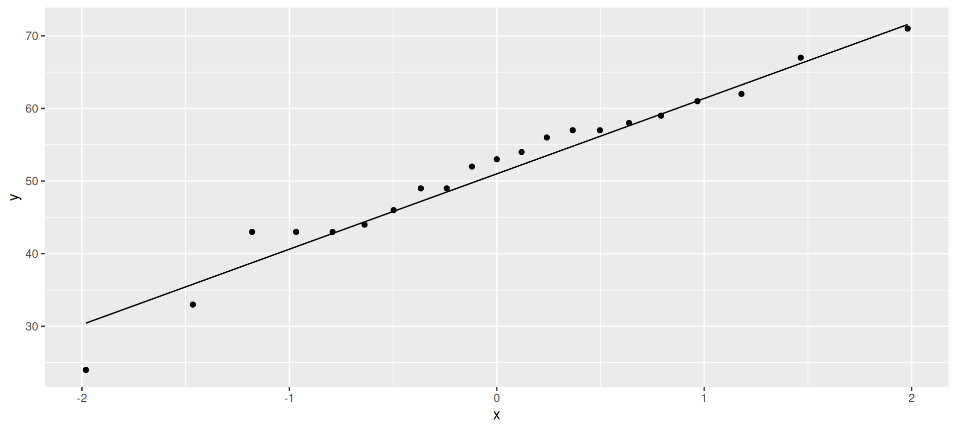
only problem here is lowest value a little too low (mild outlier).
Control group
ggplot(control, aes(sample = score)) +
  stat_qq() + stat_qq_line()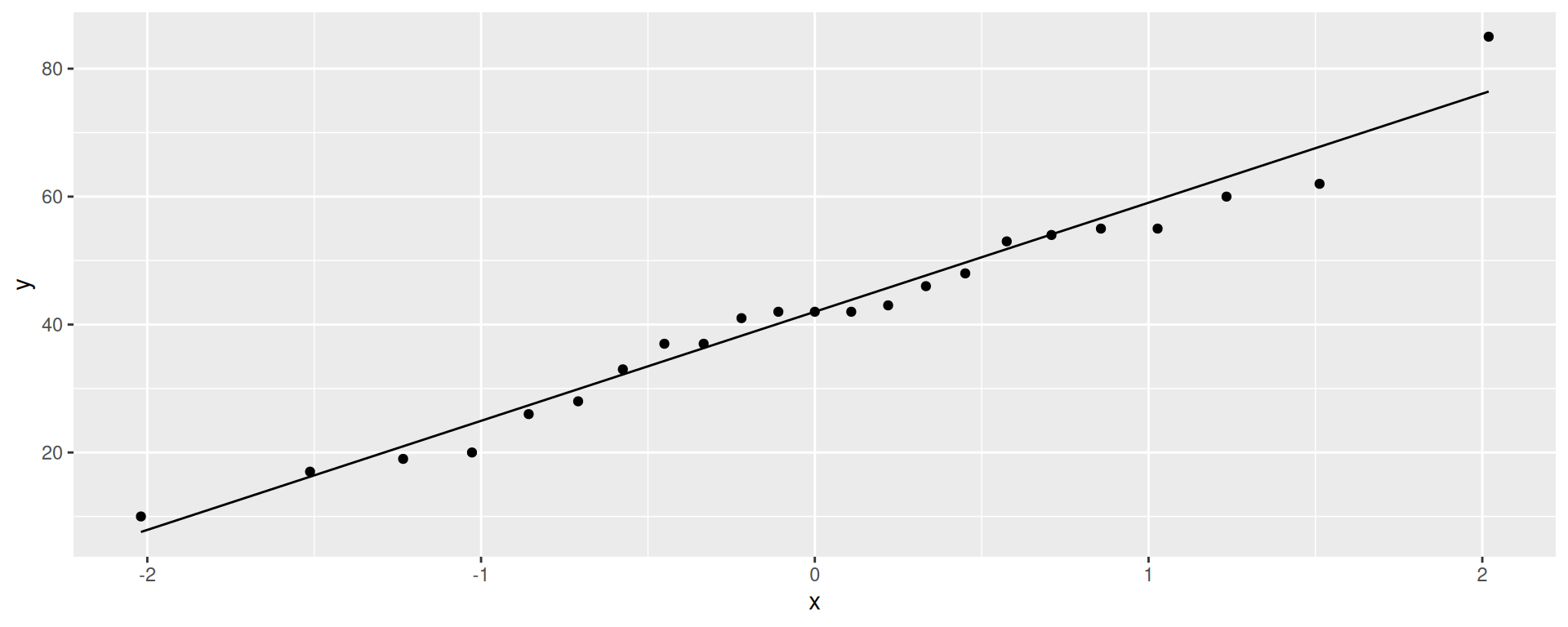
This time, highest value a little too high, but again, no real problem with normality.
Facetting more than one sample
Use the whole data set and facet by groups
ggplot(kids, aes(sample = score)) +
  stat_qq() + stat_qq_line() + facet_wrap(~group)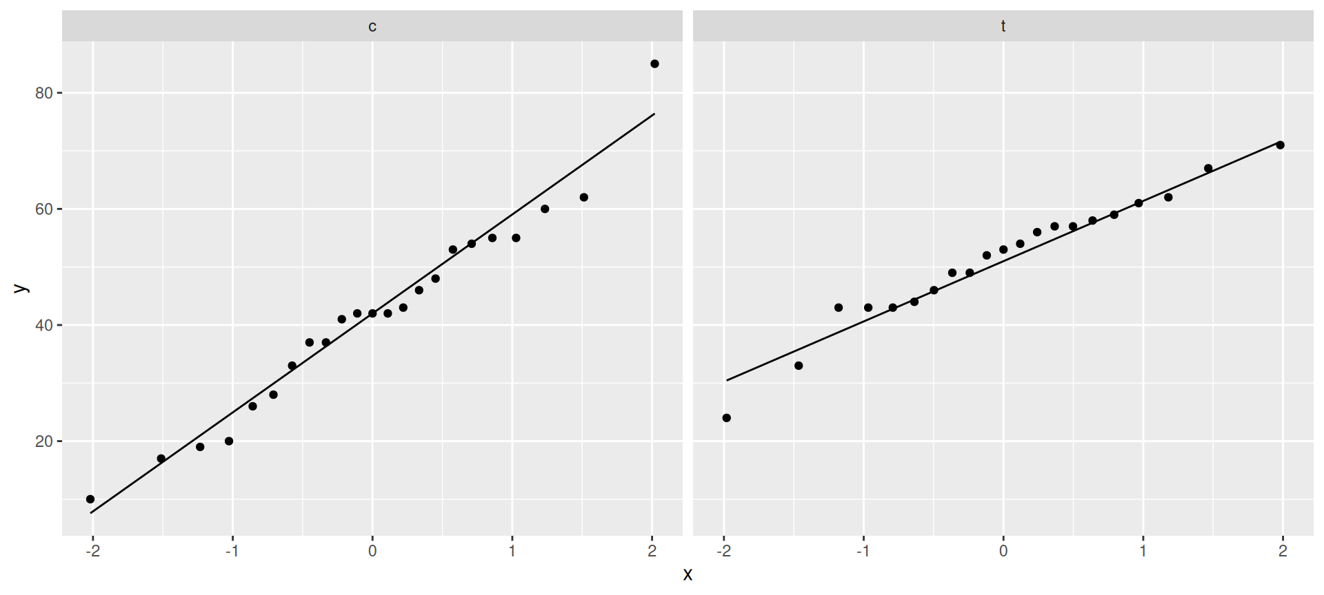
Blue Jays attendances, skewed to right
ggplot(jays, aes(x = attendance)) + geom_histogram(bins = 6)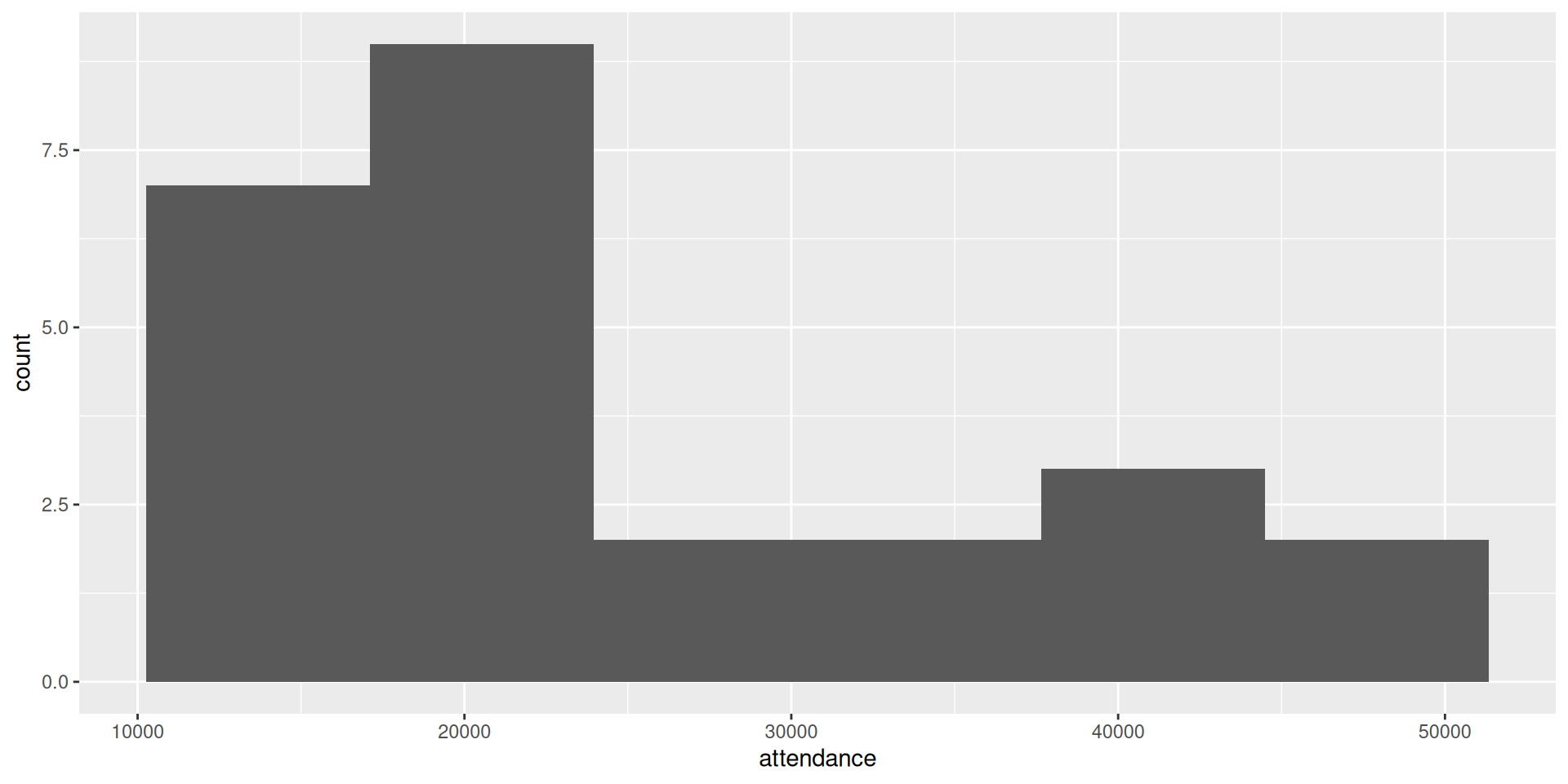
On a normal quantile plot
ggplot(jays, aes(sample = attendance)) +
  stat_qq() + stat_qq_line()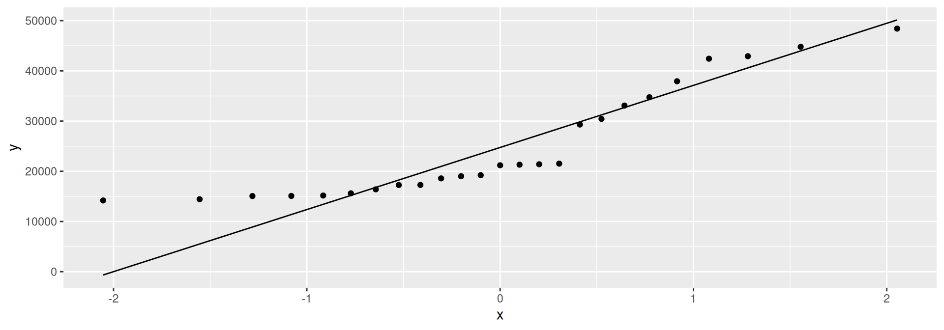
- Attendances at low end too bunched up: skewed to right.
- Right-skewness can also show up as highest values being too high, or as a curved pattern in the points.
More normal quantile plots
- How straight does a normal quantile plot have to be?
- There is randomness in real data, so even a normal quantile plot from normal data won’t look perfectly straight.
- With a small sample, can look not very straight even from normal data.
- Looking for systematic departure from a straight line; random wiggles ought not to concern us.
- Look at some examples where we know the answer, so that we can see what to expect.
Normal data, large sample
d <- tibble(x=rnorm(200))
ggplot(d, aes(x=x)) + geom_histogram(bins=10)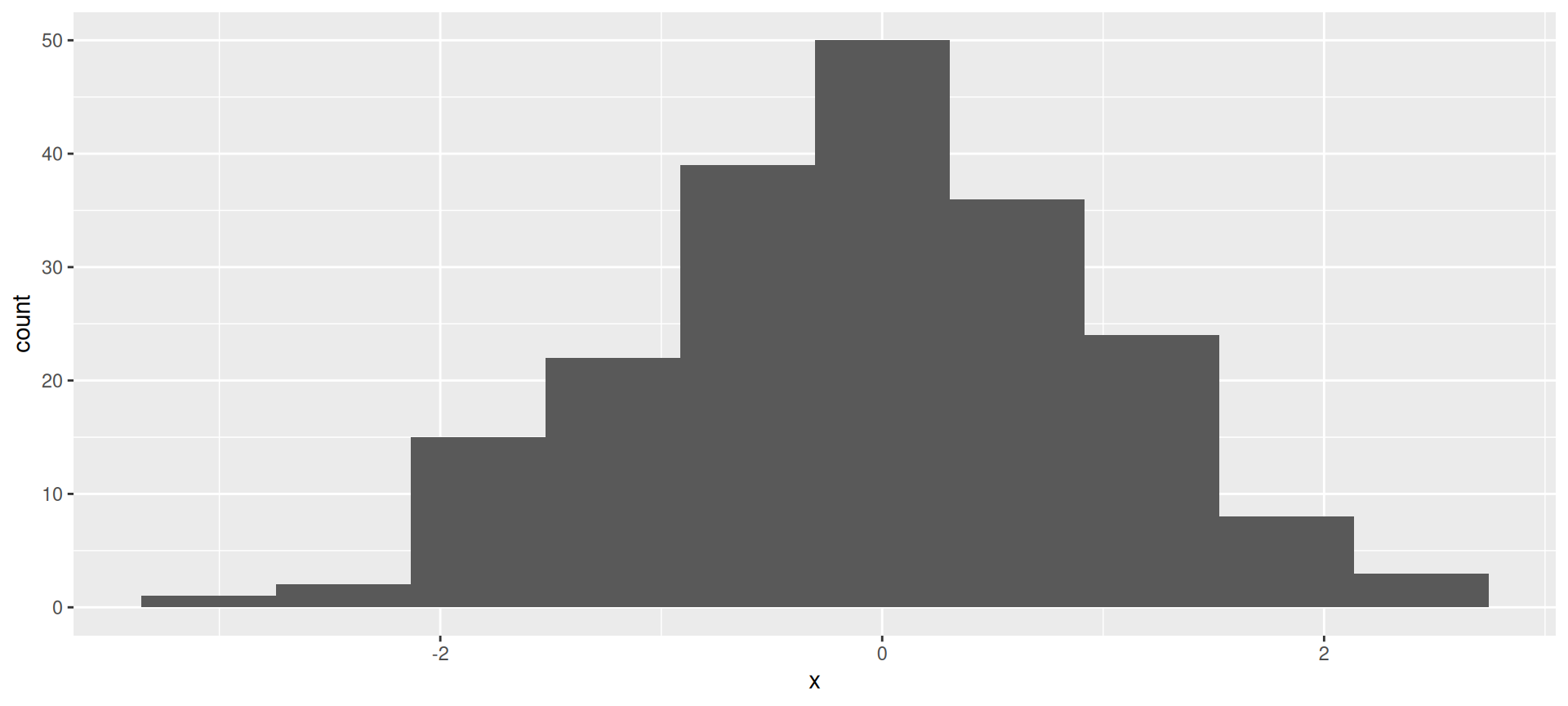
The normal quantile plot
ggplot(d,aes(sample=x))+stat_qq()+stat_qq_line()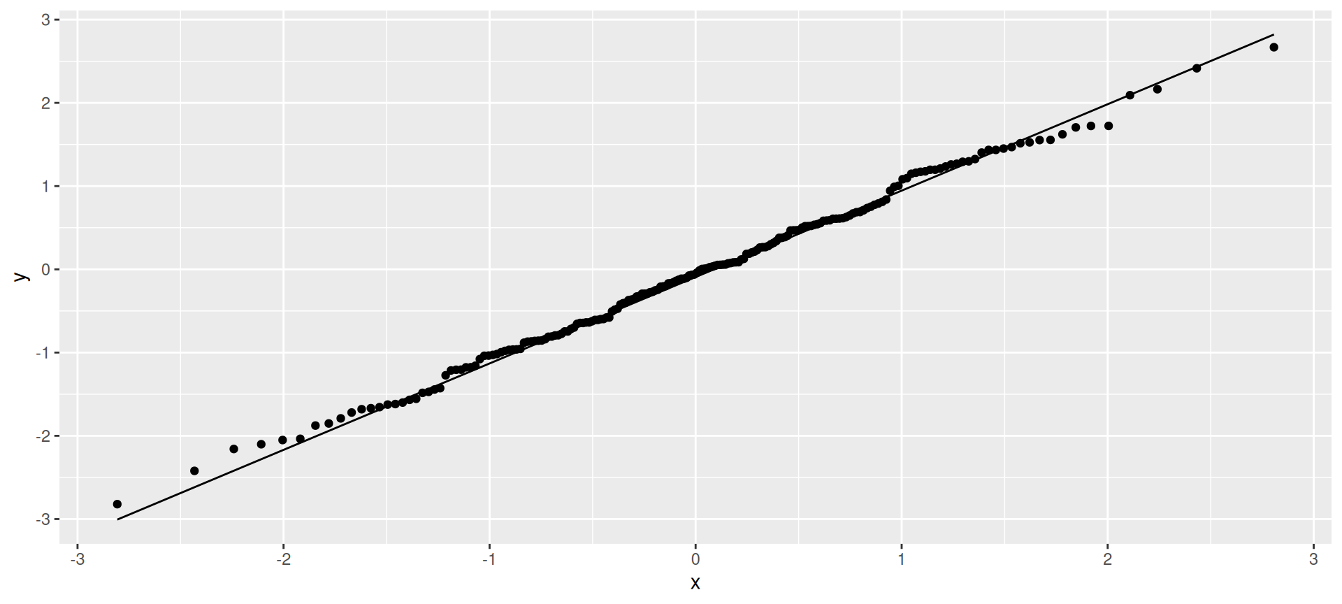
Normal data, small sample
- Not so convincingly normal, but not obviously skewed:
d <- tibble(x=rnorm(20))
ggplot(d, aes(x=x)) + geom_histogram(bins=5)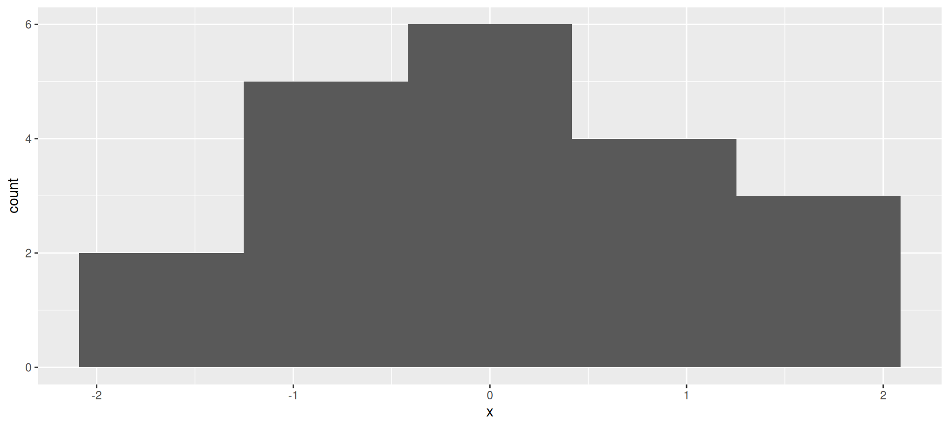
The normal quantile plot
Good, apart from the highest and lowest points being slightly off. I’d call this good:
ggplot(d, aes(sample=x)) + stat_qq() + stat_qq_line()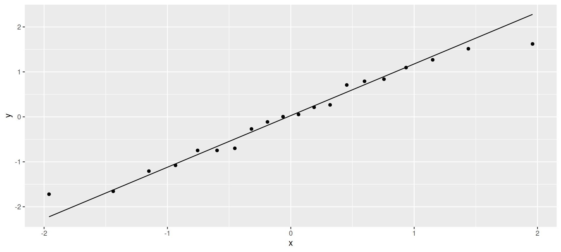
Chi-squared data, df = 10
Somewhat skewed to right:
d <- tibble(x=rchisq(100, 10))
ggplot(d,aes(x=x)) + geom_histogram(bins=10)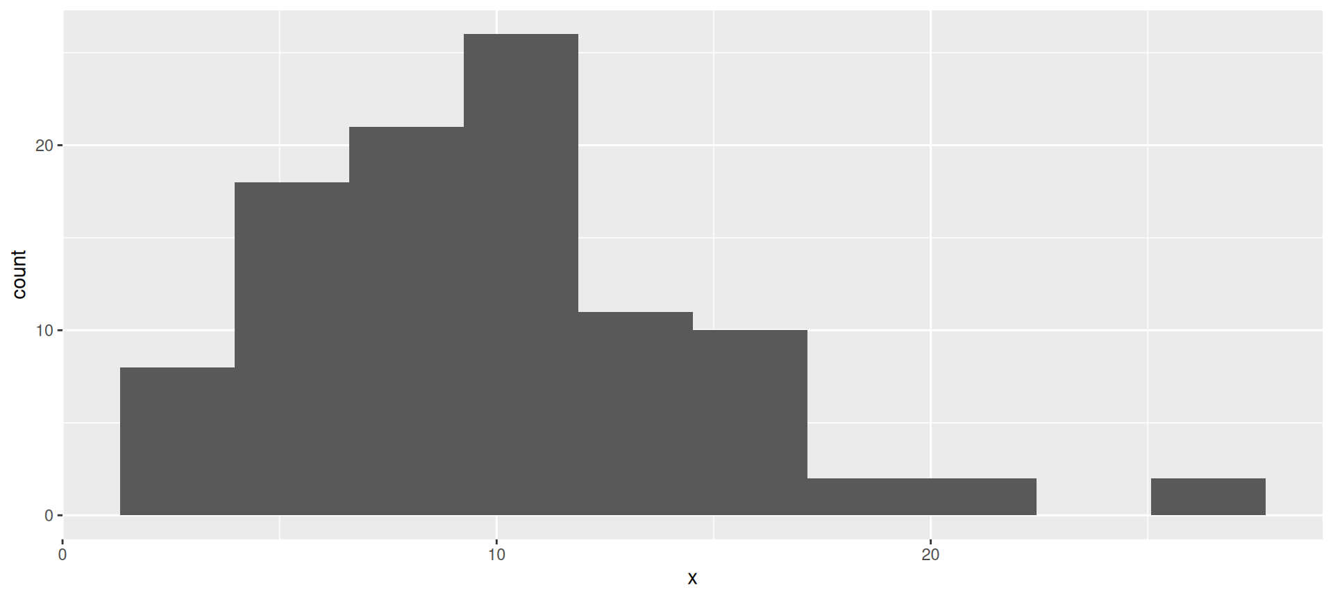
The normal quantile plot
Somewhat opening-up curve:
ggplot(d,aes(sample=x))+stat_qq()+stat_qq_line()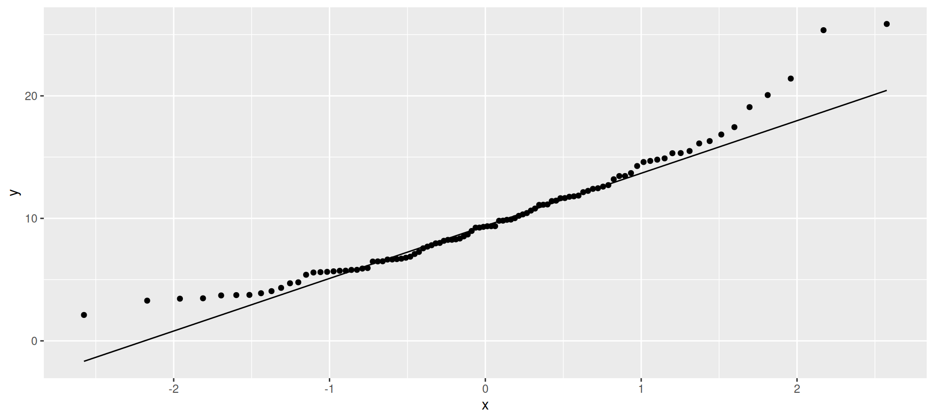
Chi-squared data, df = 3
Definitely skewed to right:
d <- tibble(x=rchisq(100, 3))
ggplot(d, aes(x=x)) + geom_histogram(bins=10)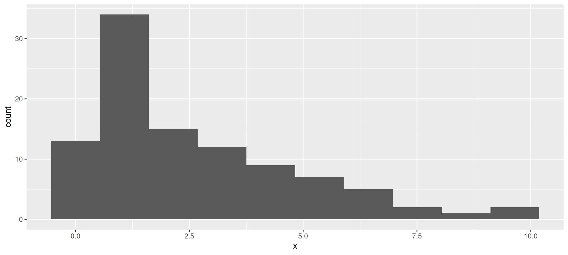
The normal quantile plot
Clear upward-opening curve:
ggplot(d,aes(sample=x))+stat_qq()+stat_qq_line()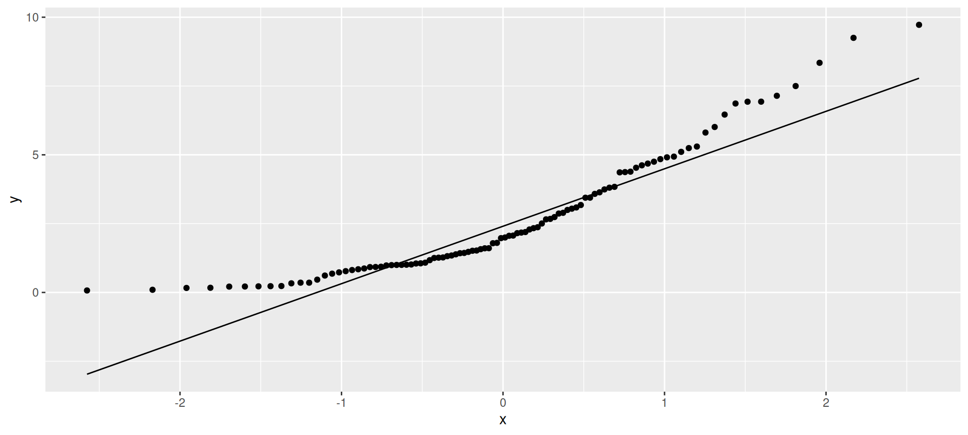
t-distributed data, df = 3
Long tails (or a very sharp peak):
d <- tibble(x=rt(300, 3))
ggplot(d, aes(x=x)) + geom_histogram(bins=15)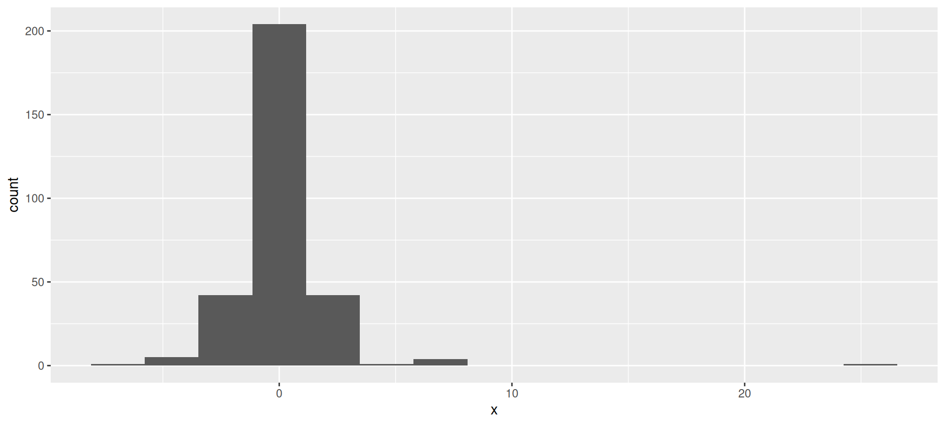
The normal quantile plot
Low values too low and high values too high for normal.
ggplot(d,aes(sample=x))+stat_qq()+stat_qq_line()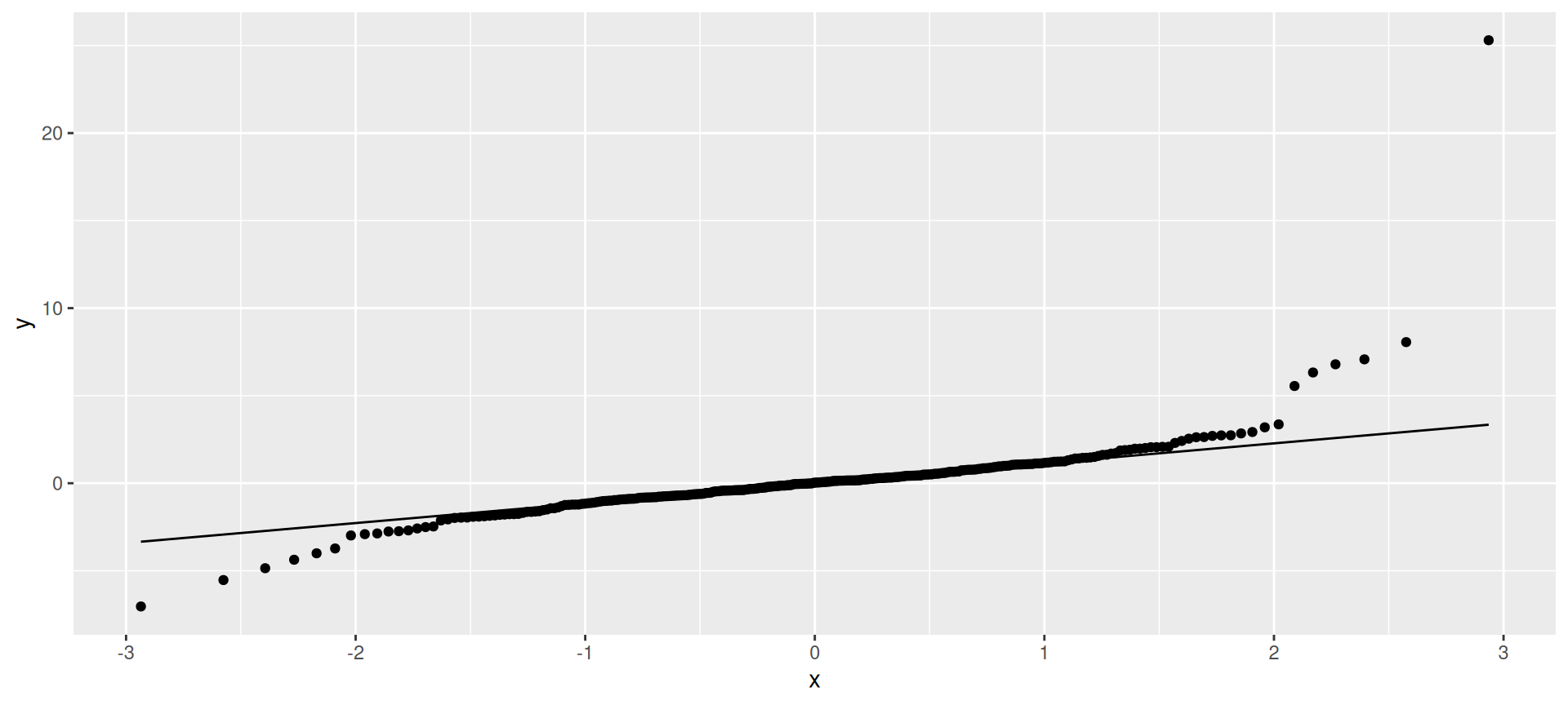
Summary
On a normal quantile plot:
- points following line (with some small wiggles): normal.
- kind of deviation from a straight line indicates kind of nonnormality:
- a few highest point(s) too high and/or lowest too low: outliers
- else see how points at each end off the line:
| High points | ||
|---|---|---|
| Low points | Too low | Too high |
| Too low | Skewed left | Long tails |
| Too high | Short tails | Skewed right |
- short-tailed distribution OK for \(t\) (mean still good), but others problematic (depending on sample size).