Drawing maps with R

Making maps in R

Spatial data comes with locations (perhaps with information about those locations).
A good way to draw spatial data is on a map.
The leaflet package is the easiest way to draw maps in R.
Install these two packages, with two familiar ones:

library(tmaptools)
library(leaflet)
library(tidyverse)
library(conflicted)
conflicts_prefer(dplyr::mutate)
conflicts_prefer(dplyr::arrange)

Hockey league map

The Ontario hockey divisions (the last example for cluster analysis) came with a very bad map. Can we do better?

reload the Ontario road distances

my_url <-
  "http://ritsokiguess.site/datafiles/ontario-road-distances.csv"
# my_url <- "ontario-road-distances.csv"
ontario <- read_csv(my_url)

Rows: 21 Columns: 22
── Column specification ────────────────────────────────────────────────────────
Delimiter: ","
chr  (1): place
dbl (21): Barrie, Belleville, Brantford, Brockville, Cornwall, Hamilton, Hun...

ℹ Use `spec()` to retrieve the full column specification for this data.
ℹ Specify the column types or set `show_col_types = FALSE` to quiet this message.

Ontario road distances (some)

ontario

# A tibble: 21 × 22
   place      Barrie Belleville Brantford Brockville Cornwall Hamilton
   <chr>       <dbl>      <dbl>     <dbl>      <dbl>    <dbl>    <dbl>
 1 Barrie          0        260       190        405      500      145
 2 Belleville    260          0       290        155      250      255
 3 Brantford     190        290         0        420      535       40
 4 Brockville    405        155       420          0       95      405
 5 Cornwall      500        250       535         95        0      500
 6 Hamilton      145        255        40        405      500        0
 7 Huntsville    125        280       300        405      450      270
 8 Kingston      330         75       340         80      180      330
 9 Kitchener     180        280        40        425      520       60
10 London        260        360        85        510      605      125
# ℹ 11 more rows
# ℹ 15 more variables: Huntsville <dbl>, Kingston <dbl>,
#   Kitchener <dbl>, London <dbl>, `Niagara Falls` <dbl>,
#   `North Bay` <dbl>, Ottawa <dbl>, `Owen Sound` <dbl>,
#   Peterborough <dbl>, Sarnia <dbl>, `Sault Ste Marie` <dbl>,
#   `St Catharines` <dbl>, `Thunder Bay` <dbl>, Toronto <dbl>,
#   Windsor <dbl>

Grab the places

and append province (“ON”) for reasons shortly to become clear:

tibble(place = ontario$place) %>% 
  mutate(prov = "ON") %>% 
  unite(place1, c(place, prov), sep = " ") -> ontario2
ontario2

# A tibble: 21 × 1
   place1       
   <chr>        
 1 Barrie ON    
 2 Belleville ON
 3 Brantford ON 
 4 Brockville ON
 5 Cornwall ON  
 6 Hamilton ON  
 7 Huntsville ON
 8 Kingston ON  
 9 Kitchener ON 
10 London ON    
# ℹ 11 more rows

Geocode 1/2

find their latitudes and longitudes (“geocode”; slow).
Save the geocoded places.

ontario2 %>% 
  rowwise() %>% 
  mutate(ll = list(geocode_OSM(place1))) -> d

# A tibble: 21 × 2
# Rowwise: 
   place1        ll              
   <chr>         <list>          
 1 Barrie ON     <named list [3]>
 2 Belleville ON <named list [3]>
 3 Brantford ON  <named list [3]>
 4 Brockville ON <named list [3]>
 5 Cornwall ON   <named list [3]>
 6 Hamilton ON   <named list [3]>
 7 Huntsville ON <named list [3]>
 8 Kingston ON   <named list [3]>
 9 Kitchener ON  <named list [3]>
10 London ON     <named list [3]>
# ℹ 11 more rows

Geocode 2/2

Untangle the lats and longs:

d %>% 
  unnest_wider(ll) %>% 
  unnest_wider(coords) -> ontario3
ontario3

# A tibble: 21 × 5
   place1        query             x     y bbox      
   <chr>         <chr>         <dbl> <dbl> <list>    
 1 Barrie ON     Barrie ON     -79.7  44.4 <bbox [4]>
 2 Belleville ON Belleville ON -77.4  44.2 <bbox [4]>
 3 Brantford ON  Brantford ON  -80.3  43.1 <bbox [4]>
 4 Brockville ON Brockville ON -75.7  44.6 <bbox [4]>
 5 Cornwall ON   Cornwall ON   -74.7  45.0 <bbox [4]>
 6 Hamilton ON   Hamilton ON   -79.9  43.3 <bbox [4]>
 7 Huntsville ON Huntsville ON -79.2  45.3 <bbox [4]>
 8 Kingston ON   Kingston ON   -76.5  44.2 <bbox [4]>
 9 Kitchener ON  Kitchener ON  -80.5  43.5 <bbox [4]>
10 London ON     London ON     -81.2  43.0 <bbox [4]>
# ℹ 11 more rows

Make map

finally:

leaflet(data = ontario3) %>% 
  addTiles() %>% 
  addCircleMarkers(lng = ~x, lat = ~y)

  # addMarkers(lng = ~x, lat = ~y)

Cluster analysis revisited

ontario %>% select(-1) %>% as.dist() -> ontario.d 
ontario.hc <- hclust(ontario.d, method = "ward.D")

Seven clusters:

plot(ontario.hc)
rect.hclust(ontario.hc, 7)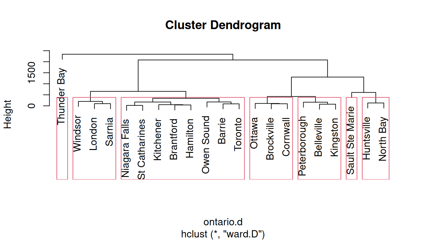

Get the clusters

tibble(place = ontario$place, cluster = cutree(ontario.hc, 7)) -> clusters
clusters %>% arrange(cluster)

# A tibble: 21 × 2
   place         cluster
   <chr>           <int>
 1 Barrie              1
 2 Brantford           1
 3 Hamilton            1
 4 Kitchener           1
 5 Niagara Falls       1
 6 Owen Sound          1
 7 St Catharines       1
 8 Toronto             1
 9 Belleville          2
10 Kingston            2
# ℹ 11 more rows

Combine clusters

combine clusters 6 and 7 with 4 (“north”)
combine clusters 2 and 3 (“east”)
make named divisions

clusters %>% 
  mutate(division = fct_collapse(factor(cluster),
                                "north" = c("4", "6", "7"),
                                "east" = c("2", "3"),
                                "west" = "5",
                                "central" = "1")) %>% 
  arrange(division) -> divisions

The divisions

divisions

# A tibble: 21 × 3
   place         cluster division
   <chr>           <int> <fct>   
 1 Barrie              1 central 
 2 Brantford           1 central 
 3 Hamilton            1 central 
 4 Kitchener           1 central 
 5 Niagara Falls       1 central 
 6 Owen Sound          1 central 
 7 St Catharines       1 central 
 8 Toronto             1 central 
 9 Belleville          2 east    
10 Brockville          3 east    
# ℹ 11 more rows

Take “ON” off of `ontario3`

ontario3 %>% 
  mutate(place = str_replace(place1, " ON$", "")) -> ontario3
ontario3

# A tibble: 21 × 6
   place1        query             x     y bbox       place     
   <chr>         <chr>         <dbl> <dbl> <list>     <chr>     
 1 Barrie ON     Barrie ON     -79.7  44.4 <bbox [4]> Barrie    
 2 Belleville ON Belleville ON -77.4  44.2 <bbox [4]> Belleville
 3 Brantford ON  Brantford ON  -80.3  43.1 <bbox [4]> Brantford 
 4 Brockville ON Brockville ON -75.7  44.6 <bbox [4]> Brockville
 5 Cornwall ON   Cornwall ON   -74.7  45.0 <bbox [4]> Cornwall  
 6 Hamilton ON   Hamilton ON   -79.9  43.3 <bbox [4]> Hamilton  
 7 Huntsville ON Huntsville ON -79.2  45.3 <bbox [4]> Huntsville
 8 Kingston ON   Kingston ON   -76.5  44.2 <bbox [4]> Kingston  
 9 Kitchener ON  Kitchener ON  -80.5  43.5 <bbox [4]> Kitchener 
10 London ON     London ON     -81.2  43.0 <bbox [4]> London    
# ℹ 11 more rows

Add the divisions, matching by place

and draw map

pal <- colorFactor("Set1", divisions$division)

ontario3 %>% left_join(divisions) %>% 
  select(place, x, y, division) %>% 
  leaflet() %>% 
  addTiles() %>% 
  addCircleMarkers(lng = ~x, lat = ~y, 
                   color = ~pal(division))

Joining with `by = join_by(place)`

Original seven clusters

The same idea gets a map of the original seven clusters:

pal <- colorFactor("Set1", divisions$cluster)
ontario3 %>% left_join(divisions) %>% 
  select(place, x, y, cluster) %>% 
  leaflet() %>% 
  addTiles() %>% 
  addCircleMarkers(lng = ~x, lat = ~y, 
                   color = ~pal(cluster))

Joining with `by = join_by(place)`

Making maps in R

Hockey league map

Ontario road distances (some)

Grab the places

Geocode 1/2

Geocode 2/2

Make map

Cluster analysis revisited

Seven clusters:

Get the clusters

Combine clusters

The divisions

Take “ON” off of ontario3

Add the divisions, matching by place

Original seven clusters

Take “ON” off of `ontario3`